Likelihoods and Observations

The previous section briefly showed you how to create random variables from prior distributions. In this section, we'll show you how to use distributions as likelihoods, to update our beliefs about those random variables based on real-world data.

Counting your Chickens

Imagine that you keep chickens, and you'd like to know the rate at which they lay eggs. You've kept track of how many you've gotten each day for the last month:

val eggs = List[Long](45, 52, 45, 47, 41, 42, 44, 42, 46, 38, 36, 35, 41, 48, 42, 29, 45, 43, 45, 40, 42, 53, 31, 48, 40, 45, 39, 29, 45, 42)

A simple model for this is to assume that the number of eggs per day is Poisson-distributed, with some mean lambda that we don't know. Since we don't know it, we should create a random variable for it. It's traditional to use a Gamma prior here.

val lambda = Gamma(0.5, 100).latent

/*
lambda: Real = Real(0.00, Infinity)
*/

Sanity check: we can see that lambda is between (0, ∞), which is good, because it doesn't make sense to lay a negative number of eggs.

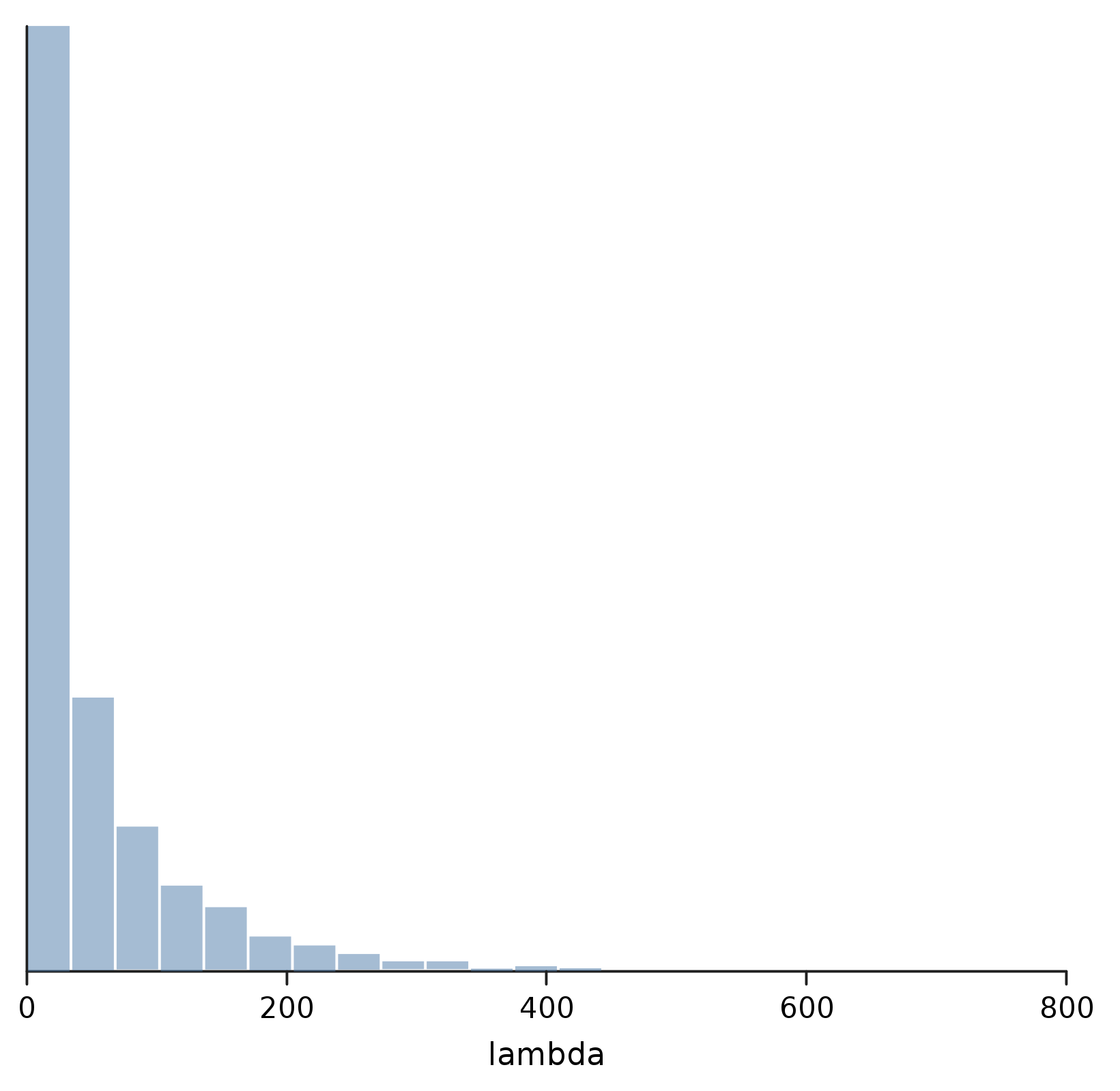
We can also confirm with a quick plot that our prior is very broad, and not very helpful for making predictions.

show("lambda", density(Model.sample(lambda)))

In fact, if we've been paying any attention to our chickens at all, we could probably have come up with a much more informative prior. But that's ok; we'll stick with the less informative one, and let the data do the talking.

Conditioning on Data

The way to connect our prior with our observations is through Model.observe. In its simplest form, it takes two parameters:

• A Seq[T] of data
• A Distribution[T] which represents the likelihood of that data

Crucially, that likelihood distribution should be parameterized by a random variable. Like this:

val eggModel = Model.observe(eggs, Poisson(lambda))

/*
eggModel: Model = Model[1]
*/

What we get back is something new: a Model object. It's printing as Model[1], which means that it's a model of a single parameter, which sounds right.

But what can we do with a Model?

Maximum a Posteriori

One thing we can do with very little ceremony is to get a single point estimate — the maximum a posteriori, or MAP — using the L-BFGS optimizer. That just looks like this:

eggModel.optimize(lambda)

/*
res1: Double = 42.00265957949004
*/

There we have, it folks: the answer to... well, our egg question, anyway.

It might seem a little bit strange that we have to pass in lambda here. After all, that's the only parameter our model has. What else could we want to find the MAP for? But Rainier tries to discourage thinking too much about the raw parameterization of a model, and instead to examine whichever random variable represents the quantites you're actually interested in. In this case, that was pretty much the same thing, but it would have been equally valid, for example, to ask for some other MAP instead:

val dozens = eggModel.optimize(lambda / 12)

/*
dozens: Double = 3.5002216316241697
*/

All well and good. But if all we wanted were point estimates, we probably wouldn't be here.

Finding a Trace

What we'd really like to do is sample the full posterior of lambda. We said that optimize is "low ceremony". Sampling, by contrast, has more steps, more to configure, and (importantly) more diagnostics to verify along the way.

The first thing we need to do is configure a sampler. For that, we'll need to import the sampler package.

import com.stripe.rainier.sampler._

What we're creating here is an EHMC, or empirical Hamiltonian Monte Carlo sampler. The 5000 warmupIterations are used to tune the sampler and find the right region to sample from; the 500 iterations will produce actual samples we'll use. There are other tuning parameters but we'll keep the defaults.

val sampler = EHMC(5000, 500)

/*
sampler: SamplerConfig = com.stripe.rainier.sampler.EHMC$$anon$1@656af720
*/

Next, we'll run the sampler on our model. What we get back is a Trace: a record of the raw parameter values produced by the sampler.

val eggTrace = eggModel.sample(sampler)

/*
eggTrace: Trace = Trace[4][500][1]
*/

By default, we run the sampler independently 4 times (4 "chains"), giving us 2000 samples in total. The Trace[4][500][1] shows us that, as well as reminding us that our model only has one parameter.

Before we keep going, we should check to make sure our sample converged. Because we ran multiple chains, we can make use of diagnostics on the trace to get back a Diagnostics(rHat, effectiveSampleSize) object for each parameter.

eggTrace.diagnostics

/*
res2: List[Trace.Diagnostics] = List(Diagnostics(0.9991309211910815, 2000.0))
*/

You can read more about rHat, the "potential scale reduction statistic", as well as effective sample size, in the Stan manual.

In this case, we've got an rHat close to the ideal value of 1, and an effective sample size that's not too far off our actual number of samples so we're looking good. If our diagnostics looked worse, we could tweak the sampler (for example giving it more warmup iterations), or we could thin out the trace, say by only keeping every other sample:

val thinTrace = eggTrace.thin(2)
thinTrace.diagnostics

/*
thinTrace: Trace = Trace[4][250][1]
res3: List[Trace.Diagnostics] = List(Diagnostics(0.9985444474592584, 814.881974772901))
*/

Plotting a Posterior

Finally, we're ready to take a look at the posterior for lambda. As with optimize, we need to specify which random variable we're interested in, by using the predict method on Trace.

val posterior = eggTrace.predict(lambda)
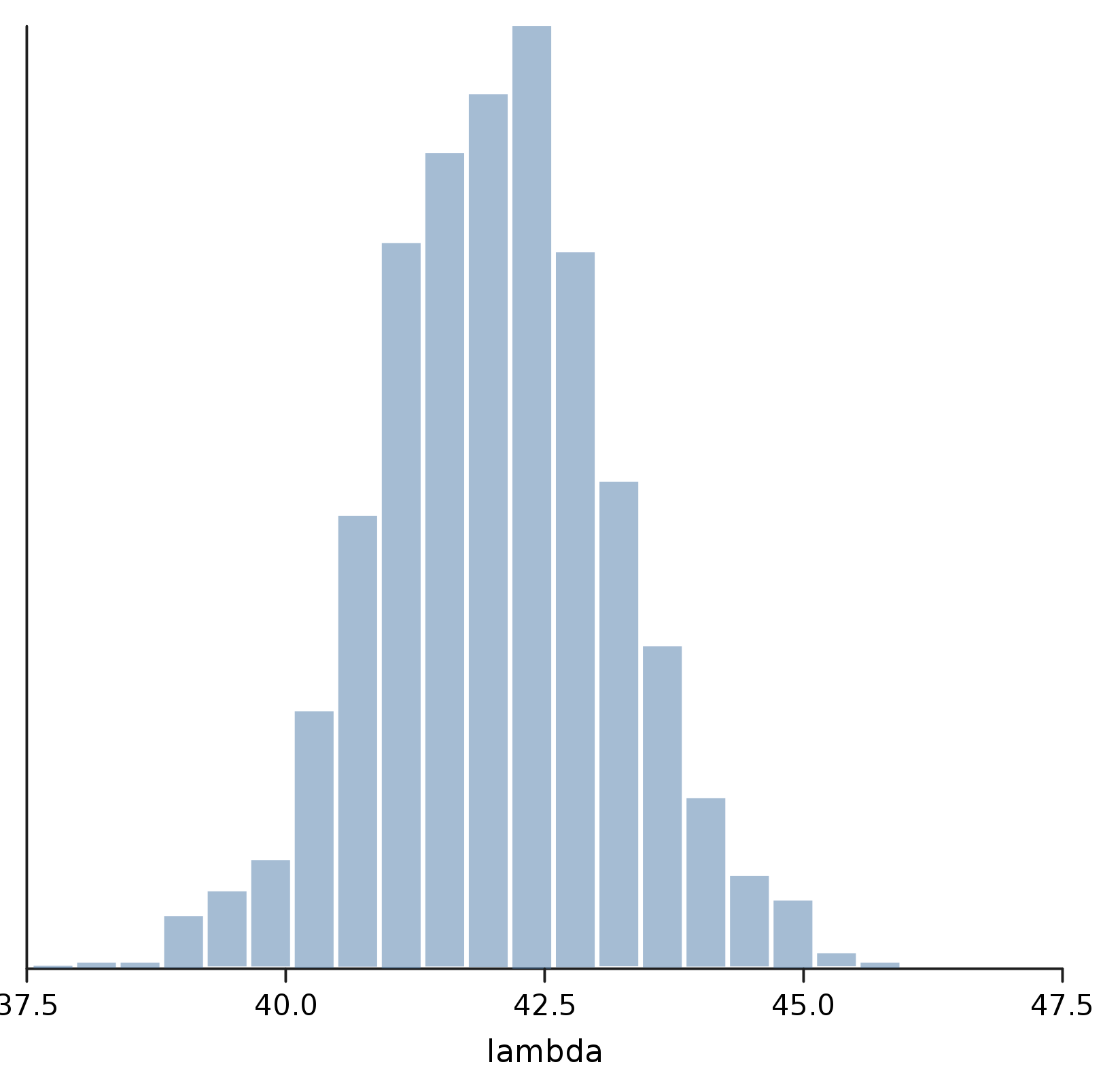
show("lambda", density(posterior))

Maybe the Answer isn't 42 after all; but we can at least be pretty confident that it's somewhere between 40 and 45.