Priors and Random Variables

Let's start by importing these two packages, which contain all of the types we will use:

import com.stripe.rainier.core._
import com.stripe.rainier.compute._

Constructing Random Variables

The most fundamental data type in Rainier is the Real, which represents a real-valued scalar random variable. A real-valued scalar is simple enough: that sounds like a Double, and indeed you can treat a Real just like a Double in a lot of ways. But since it's a random variable, it represents a set of possible values rather than one specific known value.

To construct a Real, we very often start with a Distribution object. For example, here we first construct a Uniform(0,1) distribution, and then use latent to create a new latent random variable, a, with that distribution as its prior.

val a = Uniform(0,1).latent
val b = a + 1

/*
a: Real = Real(0.00, 1.00)
b: Real = Real(1.00, 2.00)
*/

Although we don't know the exact value, you can see in the output that Rainier is tracking the bounds of each Real, as best it can: we know that a must be in the range (0,1), which means b must be within (1,2). Seeing these bounds can be a good basic sanity check as you're building a model.

You can combine Reals using normal arithmetic operations, and they support a wide range of unary operators like abs, exp, log, and logit. You can also use a Real for any parameter of a Distribution. So, for example, we can use our b and a as the mean and standard deviation of a new Normal latent variable.

val c = Normal(b, a).latent

/*
c: Real = Real(-Infinity, Infinity)
*/

Sampling from the Prior

The bounds for c are not that helpful: in theory, it can take on any real value. Some values, however, are much more likely than others. To get a view into that, we can sample from c. In fact, we can jointly sample from a and c to get a sense of not just what values are more and less likely for them, but how those values are related to each other.

We'll see a more thorough treatment of sampling later on, but for now, we can use a simple convenience method that's perfect for this kind of exploratory work.

Model.sample((a,c)).take(10)

/*
res0: List[(Double, Double)] = List(
  (0.6156257013298864, 1.095372215976534),
  (0.6055193504418845, 1.1657928784338316),
  (0.6513162868186462, 1.8960333440701265),
  (0.6117323232691895, 0.9805336083328635),
...
*/

You can see a few things here: the sampling process has converted our (a, c) tuple into a list of concrete (Double, Double) tuples. Each of those tuples is an independent joint sample of the (Real, Real) 2-dimensional random variable. We can verify that the values for a are all in that (0,1) range we expected, and that the values for c are a little more widely spread. But to get a better understanding, we should look at a plot.

Visualizing Samples

Rainier comes with plotting support, based on EvilPlot, in a separate rainier-notebook module.

NOTE: this currently is only supported for Scala 2.12.

Importing the package exposes all of the plotting methods:

import com.stripe.rainier.notebook._

Now we can create and render a basic scatter plot of our (a,c) tuples.

val ac = Model.sample((a,c)))
show("a", "c", scatter(ac))

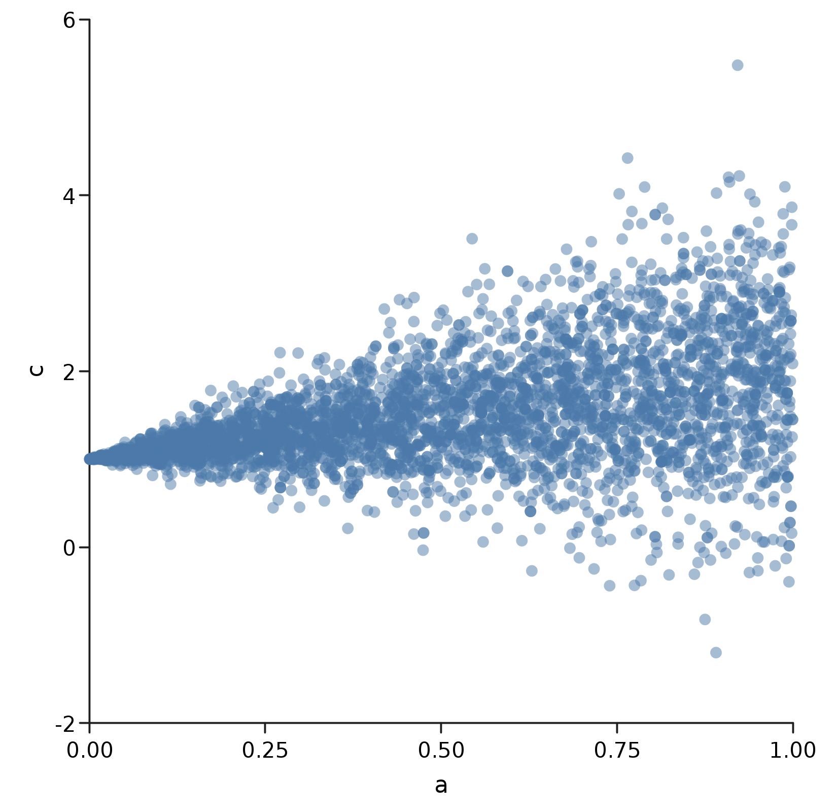Here, the relationship is a lot clearer! Because we used a as the standard deviation for c, we get a funnel shape where c spreads out more as a gets larger. But we also see that the center of the funnel shifts upwards as a grows, because we set the mean to be b = a + 1.